Applying a filter to a time-series

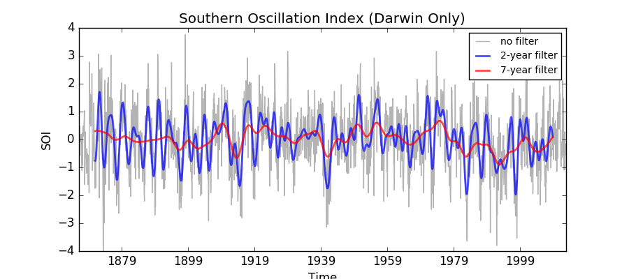
This example demonstrates low pass filtering a time-series by applying a weighted running mean over the time dimension.

The time-series used is the Darwin-only Southern Oscillation index (SOI), which is filtered using two different Lanczos filters, one to filter out time-scales of less than two years and one to filter out time-scales of less than 7 years.

References

Duchon C. E. (1979) Lanczos Filtering in One and Two Dimensions. Journal of Applied Meteorology, Vol 18, pp 1016-1022.

Trenberth K. E. (1984) Signal Versus Noise in the Southern Oscillation. Monthly Weather Review, Vol 112, pp 326-332

"""
Applying a filter to a time-series
==================================

This example demonstrates low pass filtering a time-series by applying a
weighted running mean over the time dimension.

The time-series used is the Darwin-only Southern Oscillation index (SOI),
which is filtered using two different Lanczos filters, one to filter out
time-scales of less than two years and one to filter out time-scales of
less than 7 years.

References
----------

    Duchon C. E. (1979) Lanczos Filtering in One and Two Dimensions.
    Journal of Applied Meteorology, Vol 18, pp 1016-1022.

    Trenberth K. E. (1984) Signal Versus Noise in the Southern Oscillation.
    Monthly Weather Review, Vol 112, pp 326-332

"""
import numpy as np
import matplotlib.pyplot as plt
import iris
import iris.plot as iplt


def low_pass_weights(window, cutoff):
    """Calculate weights for a low pass Lanczos filter.

    Args:

    window: int
        The length of the filter window.

    cutoff: float
        The cutoff frequency in inverse time steps.

    """
    order = ((window - 1) // 2) + 1
    nwts = 2 * order + 1
    w = np.zeros([nwts])
    n = nwts // 2
    w[n] = 2 * cutoff
    k = np.arange(1., n)
    sigma = np.sin(np.pi * k / n) * n / (np.pi * k)
    firstfactor = np.sin(2. * np.pi * cutoff * k) / (np.pi * k)
    w[n-1:0:-1] = firstfactor * sigma
    w[n+1:-1] = firstfactor * sigma
    return w[1:-1]


def main():
    # Enable a future option, to ensure that the netcdf load works the same way
    # as in future Iris versions.
    iris.FUTURE.netcdf_promote = True

    # Load the monthly-valued Southern Oscillation Index (SOI) time-series.
    fname = iris.sample_data_path('SOI_Darwin.nc')
    soi = iris.load_cube(fname)

    # Window length for filters.
    window = 121

    # Construct 2-year (24-month) and 7-year (84-month) low pass filters
    # for the SOI data which is monthly.
    wgts24 = low_pass_weights(window, 1. / 24.)
    wgts84 = low_pass_weights(window, 1. / 84.)

    # Apply each filter using the rolling_window method used with the weights
    # keyword argument. A weighted sum is required because the magnitude of
    # the weights are just as important as their relative sizes.
    soi24 = soi.rolling_window('time',
                               iris.analysis.SUM,
                               len(wgts24),
                               weights=wgts24)
    soi84 = soi.rolling_window('time',
                               iris.analysis.SUM,
                               len(wgts84),
                               weights=wgts84)

    # Plot the SOI time series and both filtered versions.
    plt.figure(figsize=(9, 4))
    iplt.plot(soi, color='0.7', linewidth=1., linestyle='-',
              alpha=1., label='no filter')
    iplt.plot(soi24, color='b', linewidth=2., linestyle='-',
              alpha=.7, label='2-year filter')
    iplt.plot(soi84, color='r', linewidth=2., linestyle='-',
              alpha=.7, label='7-year filter')
    plt.ylim([-4, 4])
    plt.title('Southern Oscillation Index (Darwin Only)')
    plt.xlabel('Time')
    plt.ylabel('SOI')
    plt.legend(fontsize=10)
    iplt.show()


if __name__ == '__main__':
    main()

(Source code, png)