 Iris 1.7
Iris 1.7
Iris builds upon interpolation schemes implemented by scipy, and other packages, to add powerful cube-aware regrid and interpolation functionality exposed through simple cube methods.
Interpolation can be achieved on a cube with the interpolate() method, with the first argument being the points to interpolate, and the second being the interpolation scheme to use. The result is a new interpolated cube.
Sample points can be defined as an iterable of (coord/coord name, value(s)) pairs (e.g. [('latitude', 51.48), ('longitude', 0)]). Whilst more interpolation schemes will become available, the only interpolation scheme currently implementing Iris’ interpolate interface is iris.analysis.Linear.
Taking the air temperature cube we’ve seen previously:
>>> air_temp = iris.load_cube(iris.sample_data_path('air_temp.pp'))
>>> print air_temp
air_temperature / (K)               (latitude: 73; longitude: 96)
     Dimension coordinates:
          latitude                           x              -
          longitude                          -              x
     Scalar coordinates:
          forecast_period: 6477 hours, bound=(-28083.0, 6477.0) hours
          forecast_reference_time: 1998-03-01 03:00:00
          pressure: 1000.0 hPa
          time: 1998-12-01 00:00:00, bound=(1994-12-01 00:00:00, 1998-12-01 00:00:00)
     Attributes:
          STASH: m01s16i203
          source: Data from Met Office Unified Model
     Cell methods:
          mean: time
We can interpolate specific values from the coordinates of the cube:
>>> sample_points = [('latitude', 51.48), ('longitude', 0)]
>>> print air_temp.interpolate(sample_points, iris.analysis.Linear())
air_temperature / (K)               (scalar cube)
     Scalar coordinates:
          forecast_period: 6477 hours, bound=(-28083.0, 6477.0) hours
          forecast_reference_time: 1998-03-01 03:00:00
          latitude: 51.48 degrees
          longitude: 0 degrees
          pressure: 1000.0 hPa
          time: 1998-12-01 00:00:00, bound=(1994-12-01 00:00:00, 1998-12-01 00:00:00)
     Attributes:
          STASH: m01s16i203
          source: Data from Met Office Unified Model
     Cell methods:
          mean: time
As we can see, the resulting cube is scalar and has longitude and latitude coordinates with the values defined in our sample points.
It isn’t necessary to specify sample points for each dimension - any dimensions which aren’t specified are preserved:
>>> result = air_temp.interpolate([('longitude', 0)], iris.analysis.Linear())
>>> print 'Original:', air_temp.summary(shorten=True)
Original: air_temperature / (K)               (latitude: 73; longitude: 96)
>>> print 'Interpolated:', result.summary(shorten=True)
Interpolated: air_temperature / (K)               (latitude: 73)
The sample points needn’t be a scalar value and may be an array of values instead. When multiple coordinates are provided with arrays instead of scalars, the coordinates on the resulting cube will be orthogonal:
>>> sample_points = [('longitude', np.linspace(-11, 2, 14)),
...                  ('latitude',  np.linspace(48, 60, 13))]
>>> result = air_temp.interpolate(sample_points, iris.analysis.Linear())
>>> print result.summary(shorten=True)
air_temperature / (K)               (latitude: 13; longitude: 14)
Interpolation in Iris is not limited to horizontal-spatial coordinates - any coordinate satisfying the prerequisites of the chosen scheme may be interpolated over.
For instance, the iris.analysis.Linear scheme requires 1D numeric, monotonic, coordinates. Supposing we have a single column cube such as the one defined below:
>>> column = iris.load_cube(iris.sample_data_path('hybrid_height.nc'))[:, 0, 0]
>>> print column.summary(shorten=True)
air_potential_temperature / (K)     (model_level_number: 15)
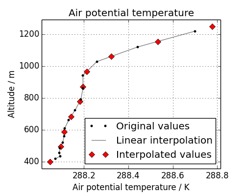
This cube has a “hybrid-height” vertical coordinate system, meaning that the vertical coordinate is unevenly spaced in altitude:
>>> print column.coord('altitude').points
[  418.7    434.57   456.79   485.37   520.29   561.58   609.21   663.21
   723.58   790.31   863.41   942.88  1028.74  1120.98  1219.61]
We could regularise the vertical coordinate by defining 10 equally spaced altitude sample points between 400 and 1250:
>>> sample_points = [('altitude', np.linspace(400, 1250, 10))]
>>> new_column = column.interpolate(sample_points, iris.analysis.Linear())
>>> print new_column.summary(shorten=True)
air_potential_temperature / (K)     (model_level_number: 10)
To see what is going on, let’s look at the original data, the interpolation line, and the new data in a plot:
As we can see with the red diamonds on the extremes of the altitude values, we have extrapolated data beyond the range of the original data. In some cases this is desirable functionality, and for others it is not - for instance, this column defined a surface altitude value of 414m, so extrapolating “air potential temperature” at 400m in this case makes little physical sense.
Fortunately we can control the extrapolation mode when defining the interpolation scheme with the extrapolation_mode keyword. For iris.analysis.Linear the extrapolation_mode must be one of linear, error, nan, mask or nanmask. To mask the values which lie beyond the range of the original data, using the mask extrapolation mode is just a matter of constructing the appropriate scheme and passing it through to the interpolate() method:
>>> scheme = iris.analysis.Linear(extrapolation_mode='mask')
>>> new_column = column.interpolate(sample_points, scheme)
The result will be a cube of the number of points passed through to interpolate, with the values requiring extrapolation being masked.
Regridding conceptually is a very similar to interpolation in Iris, with the primary difference being that interpolations are based on sample points, where regridding is based on the spatial grid of another cube.
Regridding is achieved with the cube.regrid() method, with the first argument being another cube which has the grid to which the cube should be interpolated onto, and the second argument being the regridding scheme to use.
The current regridding schemes available are iris.analysis.Linear for a linear point based regrid and iris.analysis.AreaWeighted for area weighted regridding.
Note
Regridding is a common operation needed to allow comparisons of data on different grids, however because of the powerful mapping functionality provided by cartopy, regridding is often not necessary if it is just for visualisation purposes.
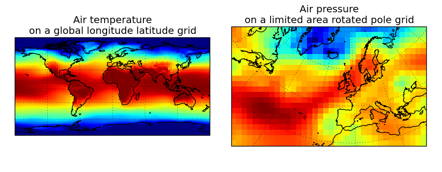
Let’s load two cubes which are on different grids:
>>> global_air_temp = iris.load_cube(iris.sample_data_path('air_temp.pp'))
>>> rotated_psl = iris.load_cube(iris.sample_data_path('rotated_pole.nc'))
We can visually confirm that they are on different grids by drawing a block plot (pcolormesh) of the two cubes:
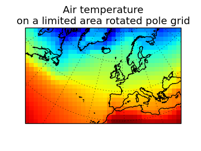
To regrid the air temperature values onto the rotated pole grid using a linear interpolation scheme, we pass the rotated_psl cube, whose grid will be used as the locations for the interpolated air temperature values:
>>> rotated_air_temp = global_air_temp.regrid(rotated_psl, iris.analysis.Linear())
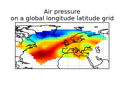
Of course, we could have interpolated the pressure values onto the global grid, but this will involve some form of extrapolation. As with interpolation, it is in the definition of the scheme where the extrapolation mode can be controlled.
When regridding the pressure cube, which is defined on a limited area rotated pole grid, on to the global grid as defined by the temperature cube, any linearly extrapolation values would quickly become dominant and highly inaccurate. We may therefore define the extrapolation_mode in the constructor of iris.analysis.Linear masking values which lie outside of the domain of the rotated pole grid:
>>> scheme = iris.analysis.Linear(extrapolation_mode='mask')
>>> global_psl = rotated_psl.regrid(global_air_temp, scheme)
Notice that, although we can still see the approximate shape of the rotated pole grid, the cells have now become rectangular in a plate-carrée/equirectangular projection, and that the resulting cube is really global, with a large proportion of the data being masked.
To conserve quantities when regridding, it is often the case that a point-based interpolation such as that provided by iris.analysis.Linear is not appropriate. The iris.analysis.AreaWeighted scheme is less general than iris.analysis.Linear, but it is a conservative regridding scheme meaning that the area weighted total is approximately preserved across grids.
With AreaWeighted, each target grid-box’s data is computed as a weighted mean of all grid-boxes from the source grid. The weighting for any given target grid-box is the area of the intersection with each of the source grid-boxes. Such a scheme is an excellent choice when regridding from a high resolution grid to a lower resolution, since all source data points will be accounted for in the target grid.
Using the same global grid we saw previously, along with a limited area cube containing total concentration of volcanic ash:
>>> global_air_temp = iris.load_cube(iris.sample_data_path('air_temp.pp'))
>>> print global_air_temp.summary(shorten=True)
air_temperature / (K)               (latitude: 73; longitude: 96)
>>>
>>> regional_ash = iris.load_cube(iris.sample_data_path('NAME_output.txt'))
>>> regional_ash = regional_ash.collapsed('flight_level', iris.analysis.SUM)
>>> print regional_ash.summary(shorten=True)
VOLCANIC_ASH_AIR_CONCENTRATION / (g/m3) (latitude: 214; longitude: 584)
One of the key limitations to the AreaWeighted regridding scheme is that the two input grids must be defined in the same coordinate system and both must contain monotonic, bounded, 1D spatial coordinates.
Note
The area weighted scheme requires spatial areas, therefore the longitude and latitude coordinates must be bounded. In this case, we can simply guess bounds based on the point values, but this step will is not necessary if the cube being worked with is already bounded:
>>> global_air_temp.coord('longitude').guess_bounds()
>>> global_air_temp.coord('latitude').guess_bounds()
Using numpy’s masked array module we can mask any data which falls below a meaningful concentration:
>>> regional_ash.data = np.ma.masked_less(regional_ash.data, 5e-6)
Finally, we can regrid the data using the area weighted scheme:
>>> scheme = iris.analysis.AreaWeighted(mdtol=0.5)
>>> global_ash = regional_ash.regrid(global_air_temp, scheme)
>>> print global_ash.summary(shorten=True)
VOLCANIC_ASH_AIR_CONCENTRATION / (g/m3) (latitude: 73; longitude: 96)
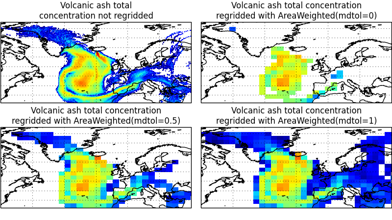
Notice how the AreaWeighted scheme allows us to define mdtol which specifies the acceptable fraction of masked data in any given target grid-box. If the fraction of masked data exceeds this value, the data in the target grid-box will be masked in the result. The fraction of masked data is calculated based on the area of masked source grid-boxes that overlaps with each target grid-box. Defining an mdtol allows fine control of masked data tolerance, but it is worth remembering that defining anything other than an mdtol of 1 will prevent the scheme from being fully conservative, as some data would be disregarded if it lies close to masked data.
To visualise the regrid, let’s plot the original data, along with 3 distinct mdtol values to compare the result: